Behind the Paper – Modeling Multiple Pathways of Carcinogenesis using the Kronecker Structure

• Splitting up mutational events in independent and dependent ones
• Building gene mutation graphs
• Using the Kronecker structure for each matrix
• Modifying parameters and initial conditions for other types of cancer
• Solving the model in a computationally feasible way
• References

How can we systematically describe the multiple pathway nature of carcinogenesis? How can we account for the fact that different types of cancer develop through different pathways which are based on different molecular parameters? Can we design a mathematical framework that can be built in a modular way and that is medically interpretable? These are some of the questions we were asking ourselves in the Mathematics in Oncology initiative. This is a collaboration between mathematicians from EMCL at Heidelberg University and HITS Heidelberg, and tumor biology experts from ATB at Heidelberg University Hospital in Germany which was initiated in 2017. It primarily focuses on the development of colorectal cancer in Lynch syndrome, the most common hereditary colorectal cancer syndrome, and its consequences on prevention, diagnosis and treatment.

Within this collaboration, we wanted to have a mathematical model of colorectal carcinogenesis that fulfills the following requirements:

1. It offers a simultaneous description of the multiple pathway nature of colorectal carcinogenesis,
2. it is modular, meaning that we can add various driver genes, mutational dependencies and whole pathways of carcinogenesis in an easy way based on current biomedical data,
3. it is medically interpretable, meaning that the parameters and components have a biomedical meaning,
4. it can be analyzed systematically, meaning that we can study the influence of different components on the evolution of cancer,
5. it is computationally feasible, meaning that even a large system can be computed quite efficiently.

In the end, we came up with the following mathematical model: a system of ordinary differential equations (ODEs) with a system matrix that is built with a specific structure, the Kronecker structure. In the following, let me explain to you what this Kronecker structure is and why it is so useful for modeling multiple pathways of carcinogenesis in a systematic way.

For this, we have to think about how to model the individual steps of the pathways of carcinogenesis, a topic which has been of interest to the mathematical oncology community for a long time (Gerstung et al., 2009; Komarova et al., 2002; Paterson et al., 2020; Tan & Brown, 1988). The steps of the pathways of carcinogenesis are typically mutational events of driver genes involved in the development of a specific type of cancer.

Let's take our example of Lynch syndrome carcinogenesis where we currently consider five possible driver genes: the classical colorectal cancer driver genes APC, KRAS, and TP53, CTNNB1, and one of the MMR genes, where the latter is quite important in Lynch syndrome carcinogenesis. In all these genes, mutational events can occur where either one mutation on one of the two alleles of one cell or two mutations on both alleles are necessary for a phenotypic change of the cell. With mutational events, we refer to point mutations or loss of heterozygosity (LOH) events.

Splitting up mutational events in independent and dependent ones

And here is the first important point: The mutational events in some genes can be independent or dependent on mutational events in other genes. Independent means that a mutation in one gene does not influence the probability for a mutation in a different gene. Dependency on the other hand refers to the fact that the mutation in one gene might make a mutation in a different gene more likely or less likely. In other words, there might be mutations which increase or decrease the probability of other mutations. If no dependency is known from data, we assume the mutations to be independent. With further research and new medical data, additional dependencies can be included into the model. Instead of modeling all these mutational processes at once, we split them into several additive components. One component (matrix $A$) for all independent mutational events and then, one component each (currently matrices $B$, $C$, $D$, $E$, and $F$) for the different dependent mutational events. Thus, adding more mutational dependencies is as easy as summing over more matrices. We end up with an ODE system where the system matrix consists of several summands:

Here, the state vector, $x(t)$, describes the mutational states of all involved genes at each time point $t$. This allows us to analyze the effect of, e.g., a specific mutational dependency on the overall carcinogenesis and we can check off requirement 4 on a systematic analysis of the individual components from above. Further, each component has a medical meaning.

Building gene mutation graphs

In the following, we will systematically build the individual matrices for independent and dependent mutational processes. In order to do so, information on the mutational states and mutational event rates of each gene is necessary. With this, we build mutation graphs consisting of vertices (red circles in Figure 1) and edges (gray arrows in Figure 1). The vertices are the mutational states of a gene and the edges are the single mutations that can happen between two mutation states. The edge weights represent the likelihood that a mutation occurs. For this, we calculate gene-specific point mutation and LOH event rates. In this sense, the parameters of the model have a medical interpretation. This, together with the interpretability of the model components, allows us to check off requirement 3 on medical interpretability from above.

An example gene mutation graph is given in Figure 1. For the classical APC-KRAS-TP53 sequence of colorectal cancer, they are also used in a mathematical model by (Paterson et al., 2020).

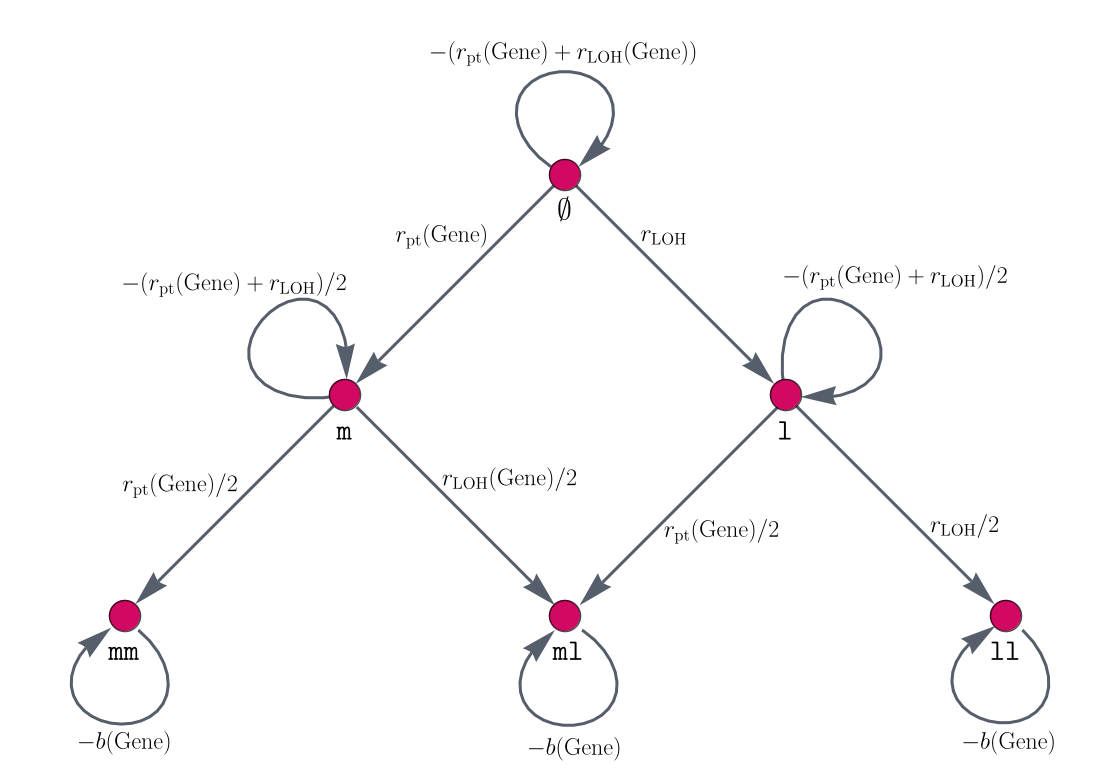
Figure 1: Gene mutation graphs. These graphs represent the possible mutation states and the connections of two subsequent mutation states. This means, the vertices represent the mutations which the alleles of a gene can have accumulated. Here, $\emptyset$ represents both alleles to be non-mutated for this gene, $\texttt{m}$ and $\texttt{mm}$ represent one respectively two alleles being hit by a point mutation, $\texttt{l}$ and $\texttt{ll}$ describe one (respectively two) alleles being affected by an LOH event, and ml is the mutation status where one allele is hit by a point mutation and the other by an LOH event. The edges connecting different vertices represent mutational events, whereas self-loops, i.e., edges that connect a vertex with itself, describe no mutation occurring at the current point in time. The edges are labeled by the amount of change which happens at each point in time.

Using the Kronecker structure for each matrix

Now you may ask yourself: ‘How can we use these gene mutation graphs to build each of the matrices $A$, $B$, $C,$ $D$, $E$, $F$ of the model? How are all these matrices defined? And where does this special matrix structure come into play?’ It is exactly at this point.

As you may have noticed, we have built these mutation graphs for each gene individually instead of building one large mutation graph of all possible combinations of mutational events for all genes at once. This can be done because of the following: First, let's consider the independent mutational events. A mutation in one gene does not affect the other mutations. This means, the mutation probabilities in one gene remain the same no matter what the mutation status in all the other genes is. You can think of this as each gene represents a coordinate axis in a Cartesian coordinate system. And this is what happens to the individual mutation graphs. They are combined using the Cartesian graph product. This huge graph now consists of all possible mutational states of all involved genes of all pathways of carcinogenesis for this type of cancer. This allows us to check off requirement 1 on describing multiple pathways of carcinogenesis simultaneously.

The graph can be written in matrix form as an adjacency matrix. And finally, here is the Kronecker structure: Combining the graphs using the Cartesian graph product leads to a large system matrix of the ODE system built by the Kronecker sum of the small adjacency matrices of the individual gene mutation graphs. This is illustrated in Figure 2.

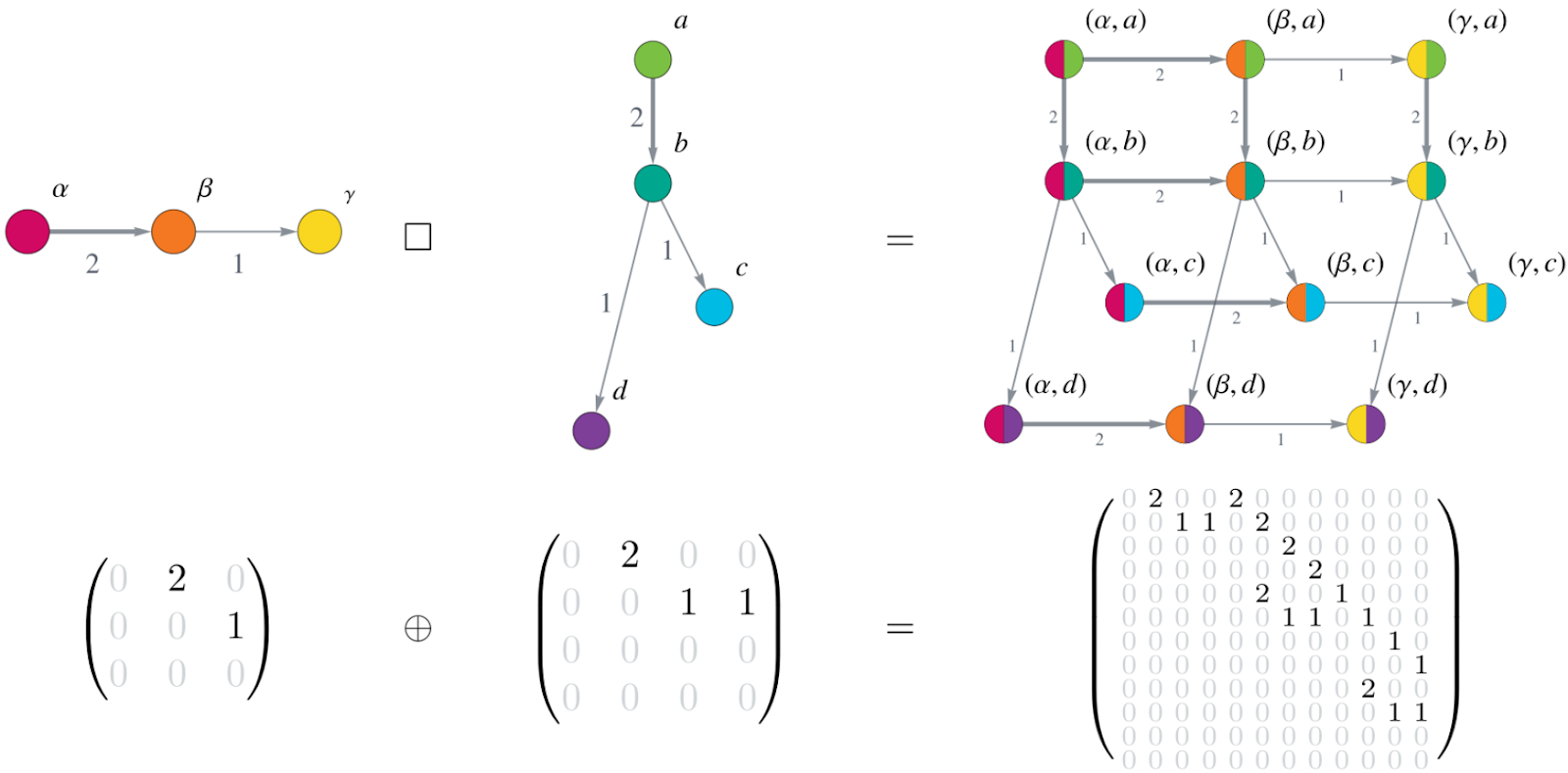
Figure 2: Cartesian product of graphs corresponds to Kronecker sum of matrices. The upper row shows two small graphs (on the left) and their Cartesian graph product (on the right). Notice how each vertex ($\alpha,\beta,\gamma$) of the first graph is combined with each vertex ($a, b, c, d$) from the second graph, yielding a total of 12 (=3$\cdot$4) vertices in the Cartesian graph product. The edge weights (indicated by numbers next to the edges and the edge thickness) of the graphs on the left and middle transfer to the corresponding edges in the product graph. The bottom row displays the adjacency matrices corresponding to the graphs in the upper row as an equation involving the Kronecker sum of the matrices.

In our model, we not only combine two matrices but five (the adjacency matrices of one of the MMR genes, of CTNNB1, APC, KRAS, and TP53 ) using the Kronecker sum. We thus end up with a matrix for the independent mutational events defined by

Adding more genes only means that the Kronecker sum includes more adjacency matrices.

And now? What about the dependent mutational events? Again, we can use the Kronecker structure because dependency refers to the correlation of a limited number of genes or events. For example, we might want to model an increased point mutation rate of one gene after a mutational event in another gene. In our case, an increased point mutation rate of APC after MMR deficiency. Or a generally increased LOH rate after the inactivation of one gene, here APC. In addition, there might be cases where two genes are hit by the same mutational event. These individual scenarios might lead to further dependencies like mutual enhancements, e.g. in our case, an APC-inactivated cell leads to an increased LOH rate. Besides that, there is the possibility of an LOH event affecting two genes simultaneously. Thus, those two dependencies enhance each other.

You can see that these biological processes can be highly complex and highly correlated. However, they can be modeled in a structured way using the Kronecker structure because, and this is very important: Although there might be a mutational dependency between some genes, all the other mutational events are not affected by this dependency. And this is the trick: You build the small mutation graph for the affected gene, e.g., for the increased point mutation rate of APC, then build the corresponding adjacency matrix, and combine it with specific diagonal matrices for the other genes indicating for which mutational states the dependency holds.

This illustrates that we can model quite complex mutational dependencies with a large number of involved genes and resulting pathways of carcinogenesis in a modular way by splitting this high-dimensional problem into small parts and combining them using the Kronecker structure.

Modifying parameters and initial conditions for other types of cancer

By the way, we can change parameters and initial conditions, to model other types of cancer. People with Lynch syndrome have an inherited germline variant in one of the MMR genes. To model the sporadic counterpart of so-called Lynch-like cancer, only the initial condition of the system has to be changed. Instead of starting with an inherited variant in one of the MMR genes in all cells, we start with non-mutated cells. Further, modeling familial adenomatous polyposis (FAP) carcinogenesis can be done by changing the initial condition of the system to an inherited variant in APC rather than in one of the MMR genes, and by adapting some parameters in the model. With this and the previously explained modular model structure, requirement 2 on modularity is satisfied.

Solving the model in a computationally feasible way

We are left with requirement 5 regarding the computational feasibility of our model. First of all, the ODE system can be solved analytically (i.e., without any approximations, which is nice for a mathematical analysis) using the matrix exponential

In our case, the system matrix $A+B+C+D+E+F$ is a sparse triangular matrix with only a few non-zero entries. In addition, we do not need to compute the matrix exponential as a full matrix. Instead, we only need the action of the matrix exponential on the vector $x_0$, where a variety of efficient algorithms exist in the context of exponential integrators (Al-Mohy & Higham, 2011; Niesen & Wright, 2012).

Moreover, if we only consider independent mutational events, the Kronecker structure can be used to also split the matrix exponential into small components. In the case of Lynch syndrome carcinogenesis, this means we only have to compute the matrix exponential of at most 6×6 matrices instead of 1250×1250 matrices. With this, also requirement 5 on computational feasibility is satisfied and thus, all requirements are fulfilled by the presented modeling approach.

As a side note, the Kronecker structure is not only very advantageous for modeling multiple pathways of carcinogenesis. It also leads to a visually quite nice fractal matrix structure, as illustrated with the Cover Art of the Math Onco Newsletter, Week 166.

Further details on the modeling approach and how it can be applied to the three pathways of colorectal Lynch syndrome carcinogenesis are available in our recent publication in PLOS Computational Biology, found here.

References